Data

Putting Youth on the Map supports data transparency and data democracy. On this page click the dropdown menu or scroll down to:

  • See our Metadata — all about our indices, data sources and their limitations
  • Download the data used in our maps
  • Find Equity Analyses — statewide analyses of the Youth Well-Being Index and Youth Vulnerability Index by sex, race/ethnicity and community type

Please refer to the original data sources for questions about data accuracy.

stockton image

Metadata

Click on a heading to view expanded information

Youth Well-Being Index (YWI)

The YWI offers a snapshot of overall youth well-being by looking across indicators of health, education, positive social relationships, and community engagement. We also break down YWI analyses by sex and race/ethnicity.
Youth Wellbeing Index graphical representation
We selected YWI indicators based on a review of research and other indices, as well as data availability for geographic units smaller than counties. For more information about the YWI, click the sections below.

I. CAUTION: YWI Data Sources and their Limitations

II. YWI Data

The YWI uses data on young people’s health, education, social relationships, and community involvement. Data types were selected based on review of research on youth well-being, review of other indices of youth well-being, and data availability. While the YWI covers some core elements of well-being, there are many important elements that we were unable to include in this index (e.g. having positive relationships with parents and other family members, support to develop a strong ethnic/cultural identity, etc.). Click each category below to learn more about YWI data.

A. Health

The Health score is based on indicators of Physical Fitness, Substance Use Avoidance and Feeling Safe.
  1. The Physical Fitness Indicator shows whether youth meet levels of fitness associated with protection against diseases linked to physical inactivity.
    1. % 9th graders deemed fit on 6 of 6 physical fitness tests (CDE)
      This measure is the percentage of youth that scored in the "Healthy Fitness Zone" for all six fitness tests: aerobic capacity, abdominal strength and endurance, upper body strength and endurance, body composition, trunk strength, and back and shoulder flexibility.
  2. The Substance Use Avoidance Indicator assess whether youth are mostly abstaining from substance use, using 3 measures from CHKS.
    1. % 9th and 11th graders who smoked 0-1 cigarettes in their lifetime (CHKS)
    2. % 9th and 11th graders who had 0-1 full drinks of alcohol in their lifetime (CHKS)
    3. % 9th and 11th graders who used marijuana 0-1 times in their lifetime (CHKS)
  3. The Feeling Safe at School Indicator assess whether youth generally feel safe at school using the mean response to a single item from CHKS.
    1. Feeling Safe at School Measure: This map shows 9th and 11th graders’ response to the question, "How safe do you feel at school?" (CHKS). Responses ranged from 1 (not very safe) to 5 (very safe).
  4. The Feeling Safe Indicator assess whether youth feel free from harassment at school based on real or perceived aspects of personal/group identity, using 6 measures from CHKS.
    1. % 9th and 11th graders not bullied at school past 12 months due to race/ethnicity/national origin (CHKS)
    2. % not bullied at school past 12 months due to religion (CHKS)
    3. % not bullied at school past 12 months due to gender (CHKS)
    4. % not bullied at school past 12 months due to sexual orientation (CHKS)
    5. % not bullied at school past 12 months due to physical or mental disability (CHKS)
    6. % not bullied at school past 12 months for other reasons (CHKS)

B. Education

The Education score is based on two indicators: High School Graduation Rate and University Readiness. For each indicator we averaged three years of data to limit effects of potential data entry errors.
  1. The High School Graduation Rate Indicator assesses whether youth are completing basic academic training, looking at the proportion of the 9th grade cohort graduating from high school (CDE).
  2. The University Ready Indicator assesses whether youth are prepared to pursue a 4-year college degree if they choose to do so, looking at the proportion of high school graduates passing state university prerequisites.

C. Social Relationships

The Social Relationships score is based on an indicator of positive relationships with adults and peers across multiple contexts, constructed by taking the mean score of 6 items that were first converted to 5-point scales.
  1. There is an adult outside school or home whom I trust (not true to very true) (CHKS)
  2. There is a teacher/other adult at my school who really cares about me (not true to very true) (CHKS)
  3. Outside home and school, there is an adult who really cares about me (not true to very true) (CHKS)
  4. I feel close to people at this school (strongly disagree to strongly agree) (CHKS)
  5. I am happy to be at this school (strongly disagree to strongly agree) (CHKS)
  6. I feel like I am part of this school (strongly disagree to strongly agree) (CHKS)

D. Community Involvement

The Community Involvement score is derived from an indicator of youth involvement in their communities outside school classes, assessed using three questions measured on a 4-point scale. The indicator is constructed by taking the mean of the 3 items.
  1. Belong to clubs, teams, church or other group activities (not true to very true) (CHKS)
  2. Involved in music, art, literature, sports, hobbies (not true to very true) (CHKS)
  3. Help other people (not true to very true) (CHKS)

III. YWI Construction and Its Limitations

For each of the four domains—health, education, social relationships, and community context—we assess the proportion of youth in the most positive category across indicators. The overall index score is an average of the four domain scores.

Click here for more on how we calculate the index.

Original data elements came in multiple forms (e.g. Likert scales of varying size, percentages). We converted each item to a percentage of the best possible score to standardize the measures. Results from correlational and principal components analyses then informed indicator construction. We use a stepwise approach in which indicators are equally weighted within each of the 4 domain scores, and then the domains are equally weighted in the overall index score.

Some of our indicators make substantial use of CHKS data. To address the challenge of low participation rates in some places (described further in the YWI Data Sources and Limitations Section), we made two choices about when to calculate the YWI.
  1. We did not calculate the Youth Well-Being Index Score for version 3 (2017) due to changes in the CHKS survey that eliminated questions used in the construction of the Social Relationships and Community Involvement domains of the YWI. The other two domains and their indicators are presented on the maps.
  2. In previous versions of the YWI, we did not calculate the Youth Well-Being Index Score for districts where CHKS participation rates were less than 40% and/or there were fewer than 15 participants who answered the survey questions used. However, underlying indicator data are provided for these districts.
  3. Analyses of the YWI and underlying CHKS indicator data are disaggregated by racial/ethnic group only when district data meet two criteria:
    • The district’s participation rate is at least 40%
    • At least 15 participants of that specific racial/ethnic background have answered the survey questions used.
Each version of the YWI uses the same data sources, but different data years. The table below lists the YWI version and years of data used for each data source. For indicators derived from CDE data, we average three years of data. Because CHKS is not administered annually, we do not average across multiple years, and use only a single year of CHKS data per district. The years of CHKS data listed for any one YWI version indicate the set of years which we draw to get data coverage for all or most districts. For example, Version 1 of the YWI uses CHKS data from 2008/09 or 2009/10, achieving nearly complete coverage across districts. Due to declines in funding for CHKS administration, fewer districts participated in later years, so we draw data from 4 years to achieve coverage of most districts in Version 2. For districts that administered CHKS more than once in that 4-year period, we use the most recent data.


Youth Wellbeing Index versions
When comparing YWI versions, it is important to remember that district boundaries change, most often as the result of district mergers. Although we account for this by aggregating data to the district boundaries as of the final year of data included in the index, districts which have experienced substantial changes between YWI versions are not directly comparable. Detailed information about district boundary changes can be found at http://www.cde.ca.gov/ds/si/ds/reorg.asp.

Like any index, the YWI presents multiple limitations (weaknesses) to consider when using results. To learn about these, please click to read the following sections.

Missing Indicators

The index lacks key indicators of well-being because data were unavailable, or unavailable at an appropriate geographic unit. For example, it does not include robust measures of relationships with parents, peers, or partners, which numerous studies find are pivotal factors in youth well-being. Nor does it include information about positive gender, ethnic and sexual identity development. Indicator data for the education domain focuses heavily on school and not at all on development of other critical life skills and knowledge (e.g. knowing how to navigate systems, manage personal finances, etc.). The analysis is also constrained by the lack of data on positive indicators of youth well-being (as opposed to measures of negative behaviors and outcomes).

Unequal Indicator Weighting

Indices are sensitive to the items included, how they are grouped, and how they are weighted in calculations of summary scores. The 'stepwise equal weighting' method used here ultimately does create unequal weights for indicators within domains due to differing numbers of indicators within a domain. Our main goals were to equally weight each area, consistent with prior research, and to ensure that indicators provided the most complete possible picture of well-being for each area. We used a method called “principal components analysis” to help avoid significant redundancy in indicator grouping and measurement of effects.

Compensatability

As with any index created by summing multiple items into a composite measure, the YWI is subject to the problem of compensatability. In brief, this means that a high score in one area may offset a low score in another, leading to a moderate overall score for an individual school district. Another school district may achieve the same overall score through the combination of moderate sub-area scores. These two districts, though qualitatively different, would appear similar on the map given their index scores. Similarly, two districts could achieve the same domain score through different combinations of values on the component indicators. The compensability problem therefore limits the ability of the index to convey how youth are faring. To help with interpretation, in the pop-up boxes associated with each district we provide information about the distribution of sub-scores whenever possible.

Inability to Test Statistical Significance

We are unable to test statistical significance between well-being scores by school districts. Since data were collected at the school district level (one observation per variable per school district) at a single point in time, we are unable to assess the stability of our estimates or the error in each observation.

Difficulty of Assessing Validity

Assessing the validity of a multidimensional index is difficult because it is unclear what criteria to use. However, a set of California Capital Region-focused qualitative studies of youth well-being (n(youth)=16, n(adult allies)=59) offered one external basis for assessment of a pilot version of the index, and patterns captured in that version did reflect local and regional qualitative descriptions (London, Erbstein et. al. 2011, available at regionalchange.ucdavis.edu/ourwork/projects/healthy-youth-healthy-regions). Going forward, it will be important to compare this index to others, assess its ability to predict various concurrent and future outcomes, and assess its utility as a tool for policy-makers, youth-focused practitioners and youth advocates.

All index construction limitations should be considered when using the YWI. Despite these limitations, the YWI captures many key aspects of youth well-being. This provides an important, although partial, snapshot of the state of California's youth.

IV. Analyzing the YWI by Sub-Groups

This website calculates and maps the YWI by sex and by racial/ethnic groups. Our approach to these analyses was constrained by the categories used by YWI data sources and CHKS participation rates and group size. Read below to learn more.

Sex Disaggregation

All sources used the categories “male” and “female,” so our analysis by sex uses them too. We only generate the YWI and domain analyses for males and females if CHKS overall participation rates are at least 40% and at least 15 individuals in the category responded to the CHKS questions we use.

Race/Ethnicity Disaggregation

YWI data sources use varying racial/ethnic categories when asking about youth racial/ethnic backgrounds. To generate the YWI and domain analyses by racial/ethnic group, we had to use categories that were applicable across all the data sources. These are: Native American/Native Alaskan (Non-Hispanic), Asian (Non-Hispanic), Filipino (Non-Hispanic), Pacific Islander/Native Hawaiian (Non-Hispanic), Black Non-Hispanic, Hispanic/Latino, White Non-Hispanic, Two or More Races. In defining these categories, we maintained as much specificity as possible, although each masks intra-group diversity.

We only generate the YWI and domain analyses for a given racial/ethnic group if CHKS overall participation rates are at least 40% and at least 15 individuals in the racial/ethnic category responded to the CHKS questions we use.

V. YWI Mapping and Its Limitations

Index data were imported into GIS software (ArcMap v10.5, ESRI, Redlands, CA) and joined to a geographic file representing merged Unified School District boundaries and Secondary School District boundaries (original boundary files downloaded from https://www.census.gov/geo/www/tiger/tgrshp2010/tgrshp2010.html). For the overall YWI, each domain (health, education, social relationships, community context) and their indicators, we designed (or “symbolized”) a map representing the data distribution. In each map, data are organized by 10% intervals that range from a low of 20% to the maximum possible score, 100%.

Note: the school district geography may still mask important intra-district geographic disparities.

All index mapping limitations should be considered when using this index.

Youth Vulnerability Index (YVI)

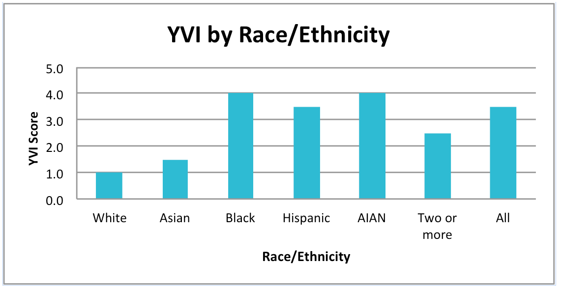
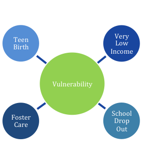
The YVI assesses vulnerability to inadequate support for well-being. It combines four types of data, which we call “indicators,”— the rates at which youth became teen mothers, did not complete high school, were placed in foster care, and lived in households with very low family incomes. The YVI and related indicator data and maps are available by county for all youth, and by race/ethnicity and sex. Data for three of the four indicators are also provided for all youth across census county divisions (CCDs). These are sub-county regions that include one or more census tracts. Data for the fourth indicator was not available at this level of geography, so we were unable to calculate the YVI for CCDs.

Youth Vulnerability Index graphical representation

Individual place-based indicator scores reflect comparison to a benchmark that could be considered excellent progress. For each indicator the benchmark is based on the rates experienced by 10% of all CA youth in the counties with the lowest rates. Each place receives a “score” for each indicator:

  1. met the benchmark
  2. somewhat below benchmark (within 90% of the benchmark)
  3. below benchmark (between 50-90% of the benchmark)
  4. far below benchmark (less than 50% of the benchmark)

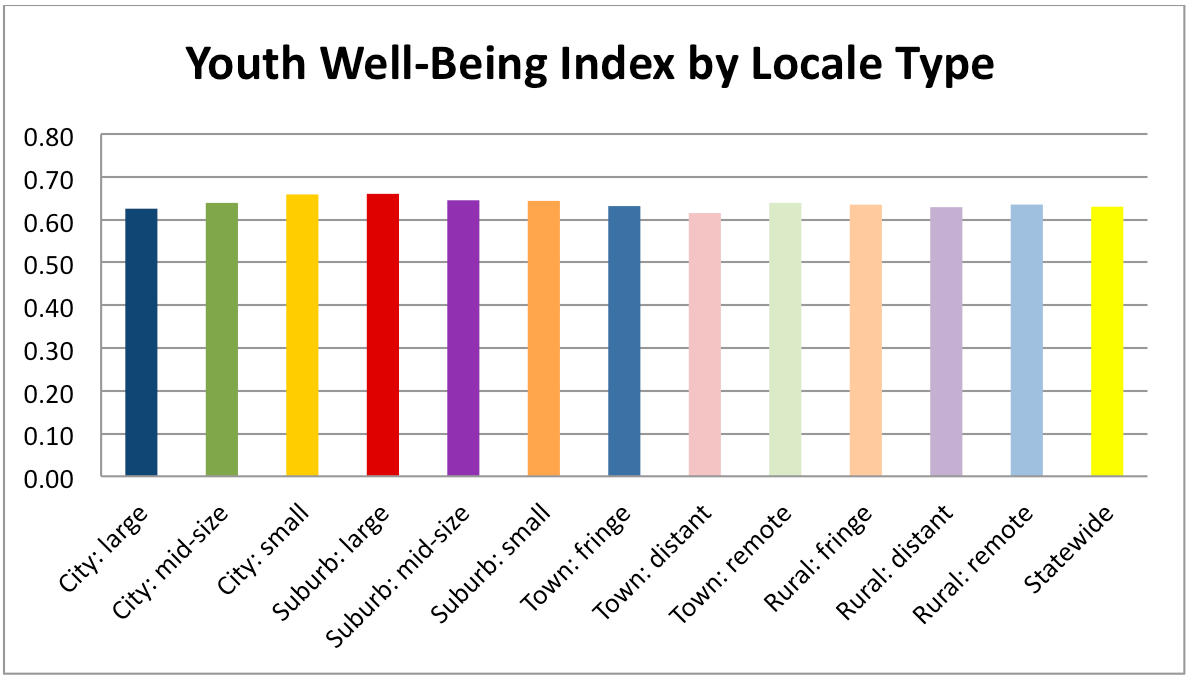
The YVI averages the four indicator scores for each county, and highlights places scoring relatively low (meaning lower vulnerability rates) and high (meaning higher vulnerability rates) across the four indicators. In counties where one or more indicators is based on an estimate that is potentially unreliable, the YVI is not calculated. Reliability concerns and thresholds are discussed in more detail below.

Many other conditions are associated with youth marginalization from potentially key institutional supports for well-being, including involvement in the juvenile justice system, teen fatherhood, identification as LGBTQ, homelessness and unauthorized immigration status. Unfortunately these data are either unavailable or unavailable in a form that can easily be mapped for the state at a sub-county level, so we are unable to include them in the index.

New Sub-Group Analysis for YVI

The YVI includes analyses by race, ethnicity and sex wherever there was an adequate population size to do so. At the county level, the YVI and its indicators are now provided for females, males, and populations identified as White, Hispanic/Latino, Black/African American, Asian, Native American/Alaskan Native, and Two or More racial/ethnic backgrounds. Due to small youth populations in many CCDs, subgroups are not analyzed separately at this geographic level. Data are provided for only three of the indicators for CCDs because foster care entry rates are not adequately geo-referenced at the sub-county level. Therefore the YVI is not calculated for CCDs.

To learn more about YVI indicator data, data sources and their limitations, click the links below.

More On YVI Calculation

To develop benchmarks for each indicator, we adopted an approach employed in health care research called “Achievable Benchmarks of Care,” or “ABC.” The basic idea is to rank order all the counties in order of performance on the indicator, and select the 90th percentile as the benchmark. This would set the benchmark at the level achieved by the county which performs better than 90% of the other counties. However, this approach can give undue influence to very small counties, which may not be very representative of the larger population. The “ABC” approach limits the influence that small places can have on the benchmark. The steps are as follows:
  1. First, calculate the performance for each county, adjusting county size to reduce the impact of smaller units
  2. rank order the counties by their adjusted performance scores
  3. beginning with the best-performing county, sequentially add county population until at least 10% of the total population is included in the sum
  4. calculate the performance for the subset of counties included in the sum by aggregating the numerator and denominator counts.
The table below shows a worked example for teen birth rate, based on a total population of 15-19 year old females in California for 2009-11 of 4,072,300.

The table lists a subset of California counties, ordered here by their adjusted teen birth rate, lowest first.

Youth Vulnerability Index
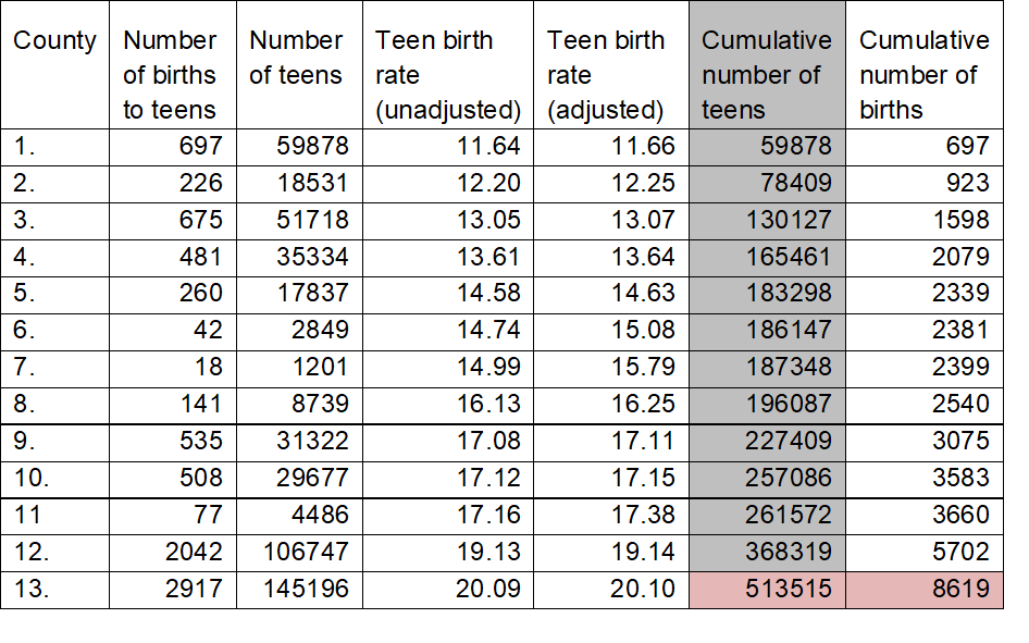
The unadjusted teen birth rate is simply the number of births to teens, divided by the number of teens, multiplied by 1,000. The adjusted teen birth rate is the number of teen births plus one, divided by the number of teens plus two, multiplied by 1,000. This adjustment has little effect in large counties, but does impact the birth rate in smaller counties. Compare the adjusted and unadjusted teen birth rates in rows 7 and 9 to see this.

After the adjusted teen birth rate is calculated, the counties are ordered by the adjusted birth rate, lowest first, as was done in the table above. The cumulative number of female teens, shown in the second to last column, crosses the 10% threshold of 407,230 in the last row, where the cumulative population is 513,515. These 13 counties are used to calculate the teen birth rate using the cumulative totals:

8619 / 513515 * 1000 = 16.78

The “ABC” benchmark for teen birth rate is thus 16.78. Counties have a teen birth rate that is 16.78 or less are given a score of 1 to indicate they met the benchmark. In the example above, counties 1 through 8 would be given a score of 1. The remaining counties, still ordered by their adjusted birth rate, are divided into 4 roughly equal-sized groups, with the first group below the benchmark assigned a score of 2, the next group assigned a score of 3, the third group assigned a score of 4, and the last group assigned a score of 5 indicating that counties in this group are well below the benchmark. The values that separate the groups in the 2010 YVI are used as benchmarks in subsequent years, permitting analysis of change in youth vulnerability over time.

Please see https://www.ncbi.nlm.nih.gov/pubmed/9828034 and https://www.ncbi.nlm.nih.gov/pubmed/10461579 for more information.

Teen Birth Rate

What do the maps show?

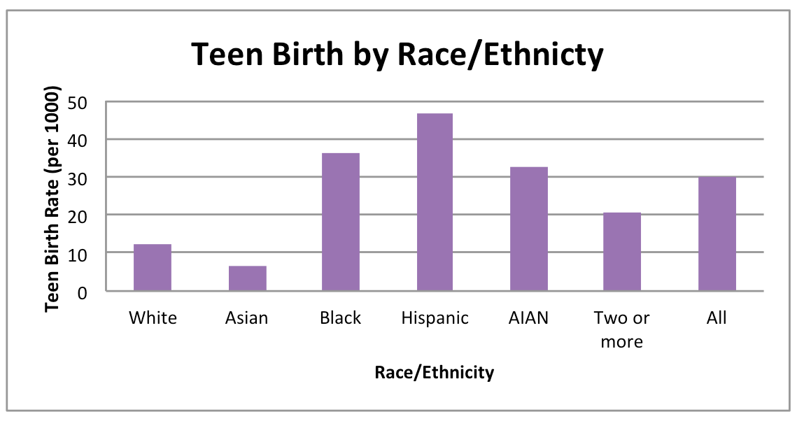
Teen mothers are more likely to not graduate from high school and/or pursue postsecondary education, experience more rapid repeat pregnancy, face the challenges of single parenting and grapple with unemployment and poverty, all of which can result in inadequate support for well-being. Teen Birth Rate maps show the number of births per 1,000 females ages 15-19. It also compares these rates to a benchmark. This benchmark is based on the teen birth rate experienced by 10% of all CA females ages 15-19 in the counties with the lowest teen birth rates. Maps by race/ethnicity are available by county only because the very small numbers of births in many CCDs make subgroup analyses unreliable.

The maps are based on estimates that are subject to uncertainty based on small population sizes or rare events. In places where estimates do not meet a certain threshold of reliability (explained below), we display an asterisk and urge you to interpret these estimates with caution as they are less likely to be accurate.

How did we calculate the teen birth rate?

This teen birth rate map represents the number of 15 to 19 year olds in each area who gave birth during the years 2009-2011, divided by the total number of females in the same age group over the same time period, multiplied by 1,000. Population totals are U.S. Census population estimates for intercensal years.

If a mother’s age or race/ethnic group was not specified, the record was dropped. For the county-level analysis, if the mother’s race was listed as “other,” the record was dropped. We used mother’s county of residence as specified in the birth records to calculate the number of births per county. For CCDs, we used mother’s residential address, geocoded to the census tract, to count the number of births to teen mothers in all census tracts within each CCD. Births that could not be geocoded were excluded (6,133 out of 128,756 births to 15 to 19 year olds, or 4.8%).

The potential for error in the estimated teen birth rate for each location depends primarily on the number of teen births. The number of teen births is expected to follow a Poisson distribution, which expresses the probability that a given number of events will occur within a fixed interval of time and space. Because there is some random temporal and spatial variability in births, the estimated birth rate may vary across geographic units or years, even when the underlying average rate is the same. A statistical measure called margin of error accounts for this naturally occurring variability, and expresses the degree of uncertainty that an estimate is close to the true value. When the margin of error is large relative to the estimate, the estimate is less reliable and should be interpreted with caution. We denote places where the margin of error is 35% the size of the estimate or larger with an asterisk. For a Poisson variable, the margin of error is equal to one divided by the square root of the number of events, multiplied by 1.645. When the number of teen births is 23 or higher, the relative margin of error falls below 35%. Therefore, the estimated birth rate in places with fewer than 23 teen births is considered unreliable and should be used with caution as the true value may differ.

For the purposes of estimating reliability, we assume that the population denominators have no error. “While this assumption is technically correct only for denominators based on the census that occurs every 10 years, the error in intercensal population estimates is usually small, difficult to measure, and therefore not considered.” (National Vital Statistics Reports, Vol. 51, No. 12, August 4, 2003, page 90 https://www.cdc.gov/nchs/data/nvsr/nvsr51/nvsr51_12.pdf).

It should be noted that population estimates for areas or groups with small populations are likely to have more variability, and teen birth estimates in these places should be used with considerable caution.

Where did we get the data?

Teen birth data were obtained (after receiving approval from the Committee for the Protection of Human Subjects) from the California Department of Public Health's Health Information and Research Section, using the Birth Statistical Master Files for 2009-11. County-level female population data came from the U.S. Census postcensal (2009) and intercensal (2010 and 2011) population estimates. Postcensal population estimates are produced by updating the resident population enumerated in a decennial census with estimates of population change (births, deaths, migration) in the years before the next decennial census. Intercensal estimates update the postcensal estimates with information from the next decennial census. We added the population estimates for 2009, 2010, and 2011 to get an estimate of the total number of females ages 15-19 for the race/ethnic groups of interest in each county. Intercensal population estimates are not available for sub-county regions, so we used data from the U.S. Census Bureau’s American Community Survey, table B11001, 5-year estimates for 2011 to get numerator data for the CCD-level teen birth rate indicator. We multiplied the ACS estimate by three to obtain an estimate of the total number of females ages 15 to 19 in in each CCD over the years 2009 to 2011.

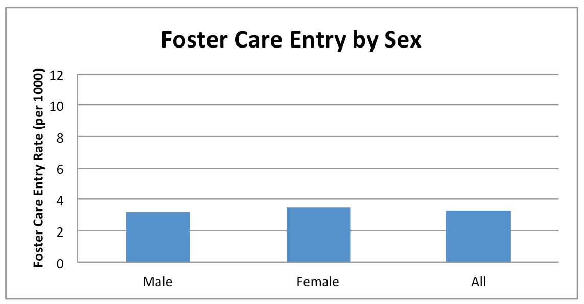
Foster Care Entry Rate

What do the maps show?

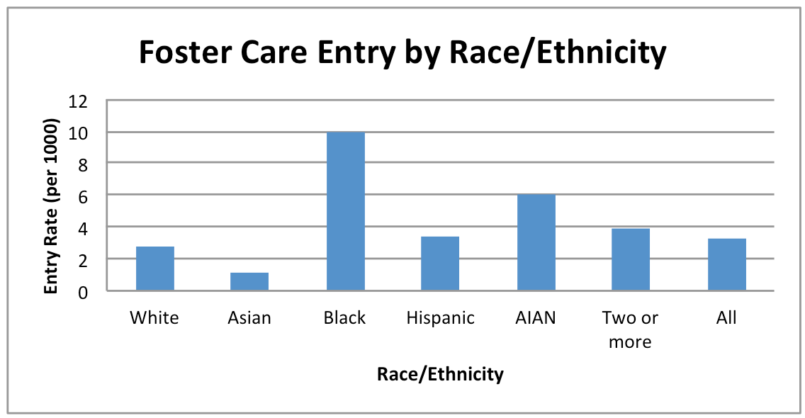
Youth who enter the foster care system tend to be vulnerable to inadequate support, which can lead to poor educational, mental and physical health, social developmental and economic outcomes. This map shows foster care entry rates per 1,000 youth age 0 to 17, for the years 2009-11. The map also compares this rate to a benchmark. This benchmark is based on the foster care entry rates experienced 10% of all CA 0-17 year olds in the counties with the lowest rates in 2009-11. Maps and data are available by county only.

The maps are based on estimates that are subject to uncertainty based on small population sizes or rare events. In places where estimates do not meet a certain threshold of reliability (explained below), we display an asterisk and urge you to interpret these estimates with caution as they are less likely to be accurate.

How did we calculate the foster care entry rate?

Foster care entry rates are the number of 0 to 17 year olds in each county who entered foster care between 2009 and 2011, divided by the number of 0-17 year olds in 2009-11, multiplied by 1,000. Foster care data could not be reliably geo-located to sub-county regions, so foster care data are not presented for CCDs.

The potential for unreliability in the foster care entry rate was assessed based on the number of foster care entries. The number of entries is expected to follow a Poisson distribution, which expresses the probability that a given number of events will occur within a fixed interval of time and space. Because there is some random temporal and spatial variability in events, the estimated foster care entry rate may vary across geographic units or years, even when the underlying average rate is the same. A statistical measure called margin of error accounts for this naturally occurring variability, and expresses the degree of uncertainty that an estimate is close to the true value. When the margin of error is large relative to the estimate, the estimate is less reliable and should be interpreted with caution. We denote places where the margin of error is 35% the size of the estimate or larger with an asterisk. For a Poisson variable, the margin of error is equal to one divided by the square root of the number of events, multiplied by 1.645. When the number of foster care entries is 23 or higher, the relative margin of error falls below 35%. Therefore, the estimated foster care entry rate in counties with fewer than 23 foster care entries is considered unreliable and should be used with caution as the true value may differ.

Where did we get the data?

Raw foster care entry data were collected from the Child Welfare Dynamic Reporting System (https://cssr.berkeley.edu/ucb_childwelfare/GeoData.aspx), a California Department of Social Services / UC Berkeley collaboration. The use agreement for these data included non-redistribution of the data. For that reason, we only allow download of the foster care entry rate rank.

Population estimates were obtained from the CA Department of Finance Demographic Unit, Report P-3: Population Projections by Race/Ethnicity, Detailed Age, and Gender, 2010-2060. (https://www.dof.ca.gov/research/demographic/reports/projections/P-3/, downloaded January 30, 2013).

Very Low Income

What do the maps show?

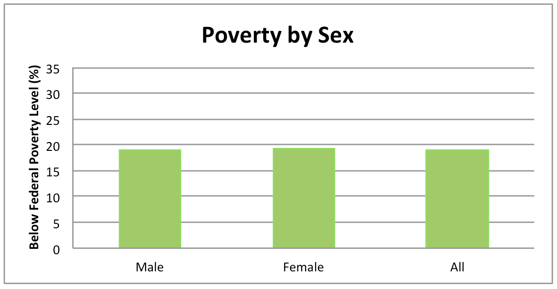
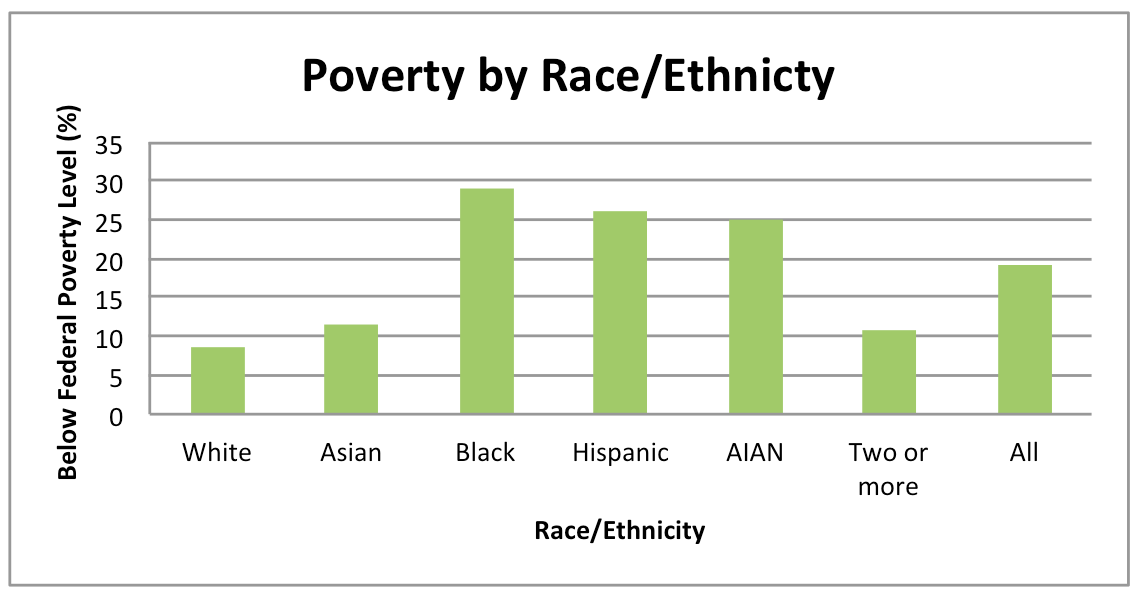
Very low family income is associated with decreased access to support for well-being. This map shows the rates at which 0 to 17 year olds are living in families with incomes that are below the federal poverty level. The map also compares this rate to a benchmark. This benchmark is based on the poverty rates experienced by 10% of all CA 0-17 year olds in the counties with the lowest poverty rates in 2010. Maps are available by sex and race/ethnicity for counties and by CCD.

The maps are based on estimates that are subject to uncertainty based on small population sizes or rare events. In places where estimates do not meet a certain threshold of reliability (explained below), we display an asterisk and urge you to interpret these estimates with caution as they are less likely to be accurate.

How did we calculate very low family income rate?

In this map we show the percentage of 0 to 17 year olds living in families with incomes that are below the federal poverty level. To generate analyses based on the benchmark, data were collected from the U.S. Census Bureau's American Community Survey 5-year estimates for 2011, using Table B17001 "Poverty Status in the Past 12 Months by Sex and Age.” Since the American Community Survey (ACS) is not a complete census, a margin of error (MOE) for each data point is given with the raw data. The margin of error is a statistical measure that represents the degree of uncertainty that a given estimate is close to the true value being estimated. When the margin of error is large relative to the estimate, the estimate is less likely to be close to the true value being estimated. We denote places where the margin of error is 35% the size of the estimate or larger with an asterisk. Please beware of large MOEs because estimates in these places are less likely to be accurate and should be interpreted with caution.

Click here for more information about the MOE calculation.

Where did we get the data?

Poverty data come from the U.S. Census Bureau’s American Community Survey table B17001, 5-year estimates.

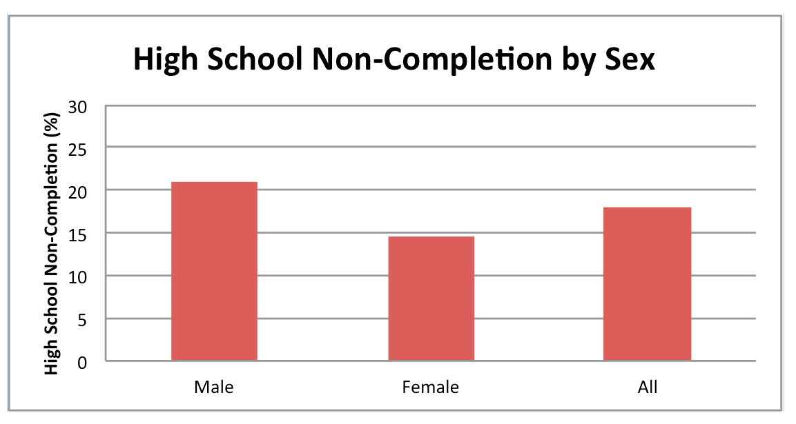
High School Non-Completion (Dropout) Rate

What does this map show?

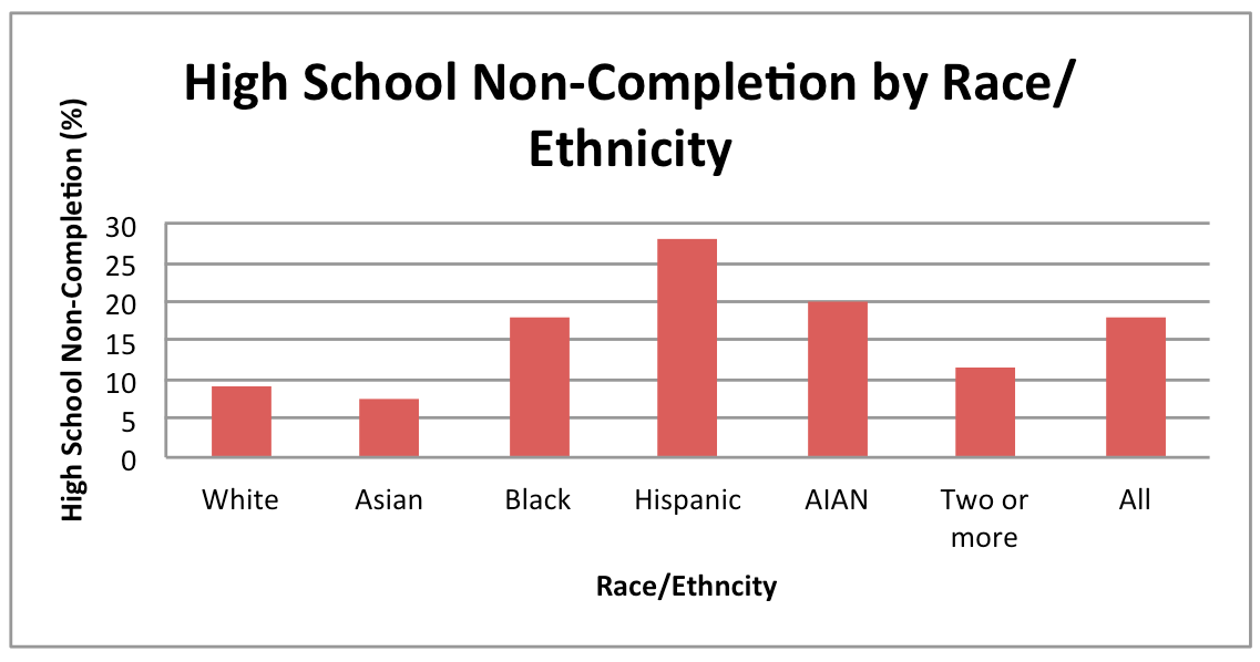
Youth who do not complete high school are more likely to experience a variety of challenges to their well-being and less access to support. This indicator measures the rates at which young people ages 18 to 24 have less than a 9th grade education or entered 9th to 12th grades but received no diploma. The map also compares this rate to a benchmark. This benchmark is based on the lowest non-completion (or “dropout”) rates experienced by 10% of all CA 18-24 year olds. Data by sex and race/ethnicity are available for counties and by CCD.

The maps are based on estimates that are subject to uncertainty based on small population sizes or rare events. In places where estimates do not meet a certain threshold of reliability (explained below), we display an asterisk and urge you to interpret these estimates with caution as they are less likely to be accurate.

How did we calculate the high school non-completion (dropout) rate?

This indicator was created by dividing the number individuals who did not complete high school by the total population of 18-24 year olds. Data were collected from the U.S. Census Bureau's American Community Survey 5-year estimates for 2007-11, using Table B15001, "Sex by Age by Educational Attainment for the Population 18 years and Over."

Since the American Community Survey (ACS) is not a complete census, a margin of error (MOE) for each data point is given with the raw data. The margin of error is a statistical measure that represents the degree of uncertainty that a given estimate is close to the true value being estimated. When the margin of error is large relative to the estimate, the estimate is less likely to be close to the true value being estimated. We denote places where the margin of error is 35% the size of the estimate or larger with an asterisk. Please beware of large MOEs because estimates in these places are less likely to be accurate and should be interpreted with caution.

Click here for more information

Where did we get the data?

To search the U.S. Census website for data, please see the American Fact Finder query tool at: https://factfinder2.census.gov/faces/nav/jsf/pages/index.xhtml.

Youth Civic Engagement

As a partner in Putting Youth on the Map, the Center for Regional Change’s California Civic Engagement Project has provided these analyses of youth (18-24 year olds) voting. Click each for detailed information about the data and analysis.

Youth Percent of the Registered Voter Population – county level analysis only

The percent of California registered voters who were youth in the 2010 general election is calculated by dividing the number of registered voters age 18-23 in that election by the total number of registered voters for each by county.

We used official registration records from each California county’s Office of the Registrar of Voters (compiled and dissaggregated by the Statewide Database). These are actual registration records and not representative samples. For more information on SWDB data collection methods, click here (https://statewidedatabase.org/data.html. Note: The Statewide Database's 2002-2012 voter data files posted on their website are currently mislabeled by age. SWDB's voter file data is actually calculated for the following age groups: ages 18-23, 24-33, 34-43, 44-53, 54-63 and 64+.

Youth Registered Voter Turnout – county and census tract level analyses

We calculated youth registered voter turnout for the 2010 general election by dividing the number of actual voters age 18-23 in that election by the number of registered voters age 18-23 for each California county and census tract.

We used official registration and voter records for all registrants from each California county’s office of the registrar of voters (compiled and disaggregated by the Statewide Database). These data are the actual voter records and not representative samples.

Youth Percent of the Vote – census tract and county level analyses

The percent of California voters who were youth in the 2010 general election is calculated by dividing the number of voters age 18-23 in that election by the total number of voters for each by county and census tract. We used voter data from the official voters records from each California county’s office of the registrar of voters (compiled and disaggregated by the Statewide Database). These data are the actual voter records and not representative samples.

Citizen Voting Age Population - county level analysis only

2010 Citizen voting age population data (those citizens age 18 and older) is from the California Department of Finance. These data estimates are the only published source of current CVAP data by age at a county level. For more information on these data, click here (https://www.dof.ca.gov/research/demographic/).

Youth Demographics

% of Population

Percentage of the Population Age 10-14

Youth population data by census tract came from the 2010 decennial census form SF1. Data downloaded at https://factfinder2.census.gov/faces/nav/jsf/pages/index.xhtml.

Percentage of the Population Age 15-19

Youth population data by census tract came from the 2010 decennial census form SF1. Data downloaded at https://factfinder2.census.gov/faces/nav/jsf/pages/index.xhtml.

Percentage of the Population Age 10-19

Youth population data by census tract came from the 2010 decennial census form SF1. Data downloaded at https://factfinder2.census.gov/faces/nav/jsf/pages/index.xhtml.

Youth Racial/Ethnic Breakdown

Latino Population

The percentage of 0 to 17 year olds who are of Latino/Hispanic origin as a percentage of the entire youth population within a county. We classified Latino/Hispanic origin based on U.S. Census data from the 2010 decennial census form SF1, P12H report. Raw data (from U.S census SF1, QTP1 report) downloaded at: https://factfinder2.census.gov/faces/nav/jsf/pages/index.xhtml.

Percentage of White Youth

The U.S. Census uses categories-- White, Black or African American, Asian, American Indian and Alaskan Native, Hawaiian and Other Pacific Islander-- to describe the racial make-up of California's young people. This map shows by county the percentage of 0 to 17 year olds that are White. County pop-ups provide a racial breakdown. Raw data from the 2010 decennial census form SF1 downloaded at https://factfinder2.census.gov/faces/nav/jsf/pages/index.xhtml.

Percentage of Black Youth

The U.S. Census uses categories-- White, Black or African American, Asian, American Indian and Alaskan Native, Hawaiian and Other Pacific Islander-- to describe the racial make-up of California's young people. This map shows by county the percentage of 0 to 17 year olds that are Black (including African Americans and other Black populations). County pop-ups provide a racial breakdown. Data came from the 2010 decennial census form SF1. Raw data from the 2010 decennial census form SF1 downloaded at: https://factfinder2.census.gov/faces/nav/jsf/pages/index.xhtml.

Percentage of Asian Youth

The U.S. Census uses categories-- White, Black or African American, Asian, American Indian and Alaskan Native, Hawaiian and Other Pacific Islander-- to describe the racial make-up of California's young people. This map shows by county the percentage of 0 to 17 year olds that are Asian. County pop-ups provide a racial breakdown. Data came from the 2010 decennial census form SF1. Raw data from the 2010 decennial census form SF1 downloaded at: https://factfinder2.census.gov/faces/nav/jsf/pages/index.xhtml.

Percentage of American Indian and Alaskan Native Youth

The U.S. Census uses categories-- White, Black or African American, Asian, American Indian and Alaskan Native, Hawaiian and Other Pacific Islander-- to describe the racial make-up of California's young people. This map shows by county the percentage of 0 to 17 year olds that are American Indian and Alaskan Native. County pop-ups provide a racial breakdown. Data came from the 2010 decennial census form SF1. Raw data from the 2010 decennial census form SF1 downloaded at: https://factfinder2.census.gov/faces/nav/jsf/pages/index.xhtml.

Percentage of Hawaiian and Other Pacific Islander Youth

The U.S. Census uses categories-- White, Black or African American, Asian, American Indian and Alaskan Native, Hawaiian and Other Pacific Islander-- to describe the racial make-up of California's young people. This map shows by county the percentage of 0 to 17 year olds that are Hawaiian and Other Pacific Islander. County pop-ups provide a racial breakdown. Data came from the 2010 decennial census form SF1. Raw data from the 2010 decennial census form SF1 downloaded at: https://factfinder2.census.gov/faces/nav/jsf/pages/index.xhtml.

Other

Click links below to see data source information and to download data.

Adequate Financial Resources

This map shows the percentage of youth ages 12-17 growing up in households earning adequate income to meet basic needs. Our threshold of "adequate" household resources draws on cost of living estimates associated with a "living wage" for families with children in California, generated by the "Living Wage Calculator" (Downloaded at https://www.livingwage.geog.psu.edu/states/06 on 3/23/11, based on the latest data available as of November 2008.); across various family configurations these estimates are approximately three times the federal poverty level. We therefore map % 12-17 year olds in households with income at least 300% federal poverty line (ACS 2012-2016 5 year estimates, Table B17024).

STDs (Gonorrhea)

The California Department of Public Health describes gonorrhea as "a common sexually transmitted infection caused by a bacterium called Neisseria gonorrhoeae. Infection can cause serious reproductive health problems, such as pelvic inflammatory disease (PID) and infertility. Gonorrhea also can cause infections in newborn babies. Tests and effective treatments are available. See below for calculation descriptions, data sources and data downloads.

Gonorrhea Rate Females Age 10-14

Here we report 2011 gonorrhea rates for females age 10 to 14 per 100,000 population. Raw data obtained from https://www.cdph.ca.gov/data/statistics/Documents/STD-Data-LHJ-DataSummaries-All.pdf.

Gonorrhea Rate Females Age 15-19

Here we report 2011 gonorrhea rates for females age 15 to 19 per 100,000 population. Raw data were obtained from https://www.cdph.ca.gov/data/statistics/Documents/STD-Data-LHJ-DataSummaries-All.pdf.

Gonorrhea Rate Males Age 10-14

Here we report 2011 gonorrhea rates for males age 10 to 14 per 100,000 population. Raw data obtained from https://www.cdph.ca.gov/data/statistics/Documents/STD-Data-LHJ-DataSummaries-All.pdf.

Gonorrhea Rate Males Age 15-19

Here we report 2011 gonorrhea rates for males age 15 to 19 per 100,000 population. Raw data obtained from https://www.cdph.ca.gov/data/statistics/Documents/STD-Data-LHJ-DataSummaries-All.pdf.

STDs (Chlamydia)

The California Department of Public Health describes chlamydia as "a common sexually transmitted infection caused by a bacterium called Chlamydia trachomatis. Infection is often without symptoms, and if not treated, can cause serious reproductive health problems such as pelvic inflammatory disease (PID) and infertility. Chlamydia also can cause infections in newborn babies. Tests and effective treatments are available." See below for calculation descriptions, data sources and data downloads.

Chlamydia Rate Females Age 10-14

Here we report 2011 chlamydia rates for females age 10 to 14 per 100,000 population. Raw data were obtained from https://www.cdph.ca.gov/data/statistics/Documents/STD-Data-LHJ-DataSummaries-All.pdf.

The dataset notation -99 means the number of cases was suppressed for confidentiality.

Chlamydia Rate Females Age 15-19

Here we report 2011 chlamydia rates for females age 15 to 19 per 100,000 population. Raw data were obtained from https://www.cdph.ca.gov/data/statistics/Documents/STD-Data-LHJ-DataSummaries-All.pdf.

The dataset notation -99 means the number of cases was suppressed for confidentiality.

Chlamydia Rate Males Age 10-14

Here we report 2011 chlamydia rates for males age 10 to 14 per 100,000 population. Raw data were obtained from https://www.cdph.ca.gov/data/statistics/Documents/STD-Data-LHJ-DataSummaries-All.pdf.

The dataset notation -99 means the number of cases was suppressed for confidentiality.

Chlamydia Rate Males Age 15-19

Here we report 2011 chlamydia rates for males age 15 to 19 per 100,000 population. Raw data were obtained from https://www.cdph.ca.gov/data/statistics/Documents/STD-Data-LHJ-DataSummaries-All.pdf.

The dataset notation -99 means the number of cases was suppressed for confidentiality.

Youth Out of Work and Out of School

Young people who are out of work and out of school often lack access to support for well-being. This map shows the “out of school/out of work” rates of 20-24 year olds for geographical areas that contain a census population of at least 100,000 people.

ACS 2006-2010 5-year estimates of 20-24 year olds who were not in school, not employed and not in the labor force were downloaded from the University of Minnesota IPUMS Program* (Integrated Public Use Microdata Series, https://usa.ipums.org/usa/index.shtml) at the PUMA level. A PUMA is a statistical geographical area that contains a census population of at least 100,000. In this analysis we used their EMPSTAT variable (which included the above selection criteria) weighted using the PERWT variable (a U.S. population weight used when doing person-level analysis).

*Steven Ruggles, J. Trent Alexander, Katie Genadek, Ronald Goeken, Matthew B. Schroeder, and Matthew Sobek. Integrated Public Use Microdata Series: Version 5.0 [Machine-readable database]. Minneapolis: University of Minnesota, 2010.

Truancy

Truancy rates in California schools for 2012-2013. CDE calculates truancy rates as the number of students with unexcused absence or tardiness on 3 or more days divided by the total enrollment (see https://www.cde.ca.gov/ls/ai/tr/ for more information about truancy). This map does NOT include truancy rates for school programs for incarcerated youth and home schools. All other school sites were geocoded using school addresses available through CDE when data were downloaded on 5/20/14.

Suspension

Food Access

The Healthy Food Financing Initiative (HFFI) Working Group has defined a food desert as, “a low-income census tract where a substantial number or share of residents has low access to a supermarket or large grocery store (see https:// www.acf.hhs.gov/programs/ocs/resource/healthy-food-financing-initiative-0). Our food access maps show the percentage and number of children ages 0 to 17 who have low access to grocery stores. Low access is defined as living more than 1/2 mile from a supermarket or large grocery store in urban tracts, and more than 10 miles from a supermarket or large grocery store in rural tracts. Low-income tracts are marked with a triangle.

Food access data were downloaded from https://www.ers.usda.gov/data-products/food-access-research-atlas/download-the-data.aspx in October 2018. For background on the food desert analysis click here. A complete data dictionary (the source of background provided) and more information on other food access analyses can be found at: https://www.ers.usda.gov/data-products/food-access-research-atlas/documentation.aspx

Transit Data

Distance to Transit Stops
This map shows the distance in meters from the population-weighted centroid of census block groups to the nearest transit stop. Data (Variable D4a) were provided by The Smart Location Database, a free data product and service provided by the U.S. EPA Smart Growth Program.(see http://www.epa.gov/smartgrowth/smartlocationdatabase.htm for original data and detailed metadata). They were not verified by UC Davis.

The U.S. EPA collected transit stop information from the General Transit Feed Specifications (https://developers.google.com/transit/gtfs/ ) in December 2012 and January 2013, and from the Transit Oriented Development Database (http://toddata.cnt.org/) , where data were updated as of 2011. EPA obtained Census block group boundaries from 2010 Census TIGER/Line shapefiles and combined them into a single national ArcGIS feature class. EPA also obtained 2010 block group “centers of population”7 from the Census. These centroids were used in geoprocessing the distance to transit stops.

Percentage of Households with 0, 1 and 2 or more cars
Vehicle ownership analyses were generated by the U.S. EPA and made available through the Smart Location Database. Auto ownership fields were derived from the ACS 2006-2010 table B25044. Percent auto ownership fields were calculated as the share of all households having zero cars (Pct_AO0), one car (Pct_AO1), or two or more cars (Pct_AO2p) with respect to total households reported in the ACS table (adapted from Ramsey, K.R. & Bell, A. (2014). Smart Location Database Version 2.0 User Guide (March 14, 2014). Washington D.C.: U.S. EPA.). EPA obtained CBG boundaries from 2010 Census TIGER/Line shapefiles and combined them into a single national ArcGIS feature class. TIGER2010_bg10 is the basic geographic dataset to which all SLD variables are appended. U.C. Davis extracted analyses from the U.S. EPA Smart Location Database in July 2014).

Transit Service Frequency
EPA analyzed GTFS data to calculate the frequency of service for each transit route between 4:00 and 7:00 PM on a weekday. Then, for each block group, EPA identified transit routes with service that stops within 0.4 km (0.25 miles). Finally EPA summed total aggregate service frequency by block group. Values for this metric are expressed as service frequency per hour of service. All block groups in areas where GTFS service data are unavailable are given the value -99999. (Adapted from Ramsey, K.R. & Bell, A. (2014). Smart Location Database Version 2.0 User Guide (March 14, 2014). Washington D.C.: U.S. EPA, p.25. For additional information on regions for which data are available, see Appendix A.)

Geographic District Boundaries

California Counties

The boundary files were downloaded from Cal-Atlas Geospatial Clearinghouse (https://atlas.ca.gov/).

Old Congressional Districts 2001

These congressional district boundaries were enacted on September 13, 2001, and signed into law on September 26, 2001 by the Governor of California. The boundary files were downloaded from Cal-Atlas Geospatial Clearinghouse (https://atlas.ca.gov/). Please note: redistricting was performed in 2011. See the New Congressional Districts 2011 map layer for changes. We do not provide a download of this boundary file.

Old State Senate Districts 2001

These state senate district boundaries were enacted on September 13, 2001, and signed into law on September 26, 2001 by the Governor of California. The boundary files were downloaded from Cal-Atlas Geospatial Clearinghouse (https://atlas.ca.gov/). Please note: redistricting was performed in 2011. See the New State Senate Districts 2011 map layer for changes. We do not provide a download of this boundary file.

Old State Assembly Districts 2001

These state assembly district boundaries were enacted on September 13, 2001, and signed into law on September 26, 2001 by the Governor of California. The boundary files were downloaded from Cal-Atlas Geospatial Clearinghouse (https://atlas.ca.gov/). Please note: redistricting was performed in 2011. See the New State Assembly Districts 2011 map layer for changes. We do not provide a download of this boundary file.

New Congressional Districts 2011

These congressional district boundaries were developed by the California Citizens Redistricting Commission (created in 2008 in response to the passage of California Proposition 11), following the passage of California Proposition 20 in 2010. They were downloaded from https://wedrawthelines.ca.gov/. Please note: We do not provide a download of this boundary file.

New State Senate Districts 2011

These state senate district boundaries were developed by the California Citizens Redistricting Commission (created in 2008 in response to the passage of California Proposition 11), following the passage of California Proposition 20 in 2010. They were downloaded from https://wedrawthelines.ca.gov/. Please note: We do not provide a download of this boundary file.

New State Assembly Districts 2011

These state assembly district boundaries were developed by the California Citizens Redistricting Commission (created in 2008 in response to the passage of California Proposition 11), following the passage of California Proposition 20 in 2010. They were downloaded from https://wedrawthelines.ca.gov/. Please note: We do not provide a download of this boundary file.

RUCA

The Rural-Urban Commuting Area Codes (RUCAs) were developed using census definitions of rural or urban status combined with work commuting information.

Urban-Rural Classification Map (2010)

This map uses US Census categories to depict census tracts as part of Urbanized Areas (at least 50,000 people), Urban Clusters (2500-49,999 people), and Rural (0-2499 people).

An urban area includes a densely settled core of census tracts and/or census blocks that meet minimum population density requirements, along with adjacent territory containing non-residential urban land uses and territory with low population density included to link outlying densely settled territory with the densely settled core. To qualify as an urban area, the territory must encompass at least 2,500 people, at least 1,500 of which reside outside institutional group quarters (e.g. prisons). The U.S. Census Bureau identifies two types of urban areas:

  • Urbanized Areas (UAs) of 50,000 or more people;
  • Urban Clusters (UCs) of at least 2,500 and less than 50,000 people.

“Rural” encompasses all population, housing, and territory not included within an urban area. For more information see https://www.census.gov/geo/reference/ua/urban-rural-2010.html. Data downloaded May 2014.

Download

Download the data by clicking on the links below. Data and data dictionaries are provided in Excel Workbooks. If you are interested in spatial data, please see the KML Files section below.

Youth Well-Being Index

Youth Vulnerability Index- County

Youth Vulnerability Index- CCD

Youth Civic Engagement

Youth Demographics

Adequate Financial Resources

Food Access

Percent Out of Work and Out of School

Sexually Transmitted Diseases

Truancy and Suspensions

Transit Access

KML files

KML (Keyhole Markup Language) is file format used to display geographic data in web-based online maps or an Earth browser such as Google Earth, Google Maps, and Google Maps for mobile. We currently provide KML files for the Youth Well-Being Index and will add more files in the future or as needed. If you have interest in obtaining a KML file not listed below, or have any questions regarding KML use, please Contact the CRC .

Dataset Year Name Description Size Download
2013 Youth Well-Being Index: All data/General population This KML provides data for all 12 indices and indicators of the Youth Well-Being Index for the "All" population category only. 52 MB PYOM_ywi_AllDataGenPop2013.zip
2013 Youth Well-Being Index: Index/Race and gender breakdown This KML provides data for the Youth Well-Being Index only, for all race and gender categories. 48 MB PYOM_ywi_Index2013.zip

Equity Analyses

The Youth Well-Being Index (YWI) and Youth Vulnerability Index (YVI) maps show index scores and indicator rates by sex and race/ethnicity for specific places. This page provides statewide analyses of the YWI and YVI. For the YWI we provide analyses by sex, race/ethnicity and community type (e.g. rural, suburban, urban). For the YVI we provide analyses by sex and race/ethnicity. These analyses use the same data and calculations as the maps; for more information about them please see the Metadata page.

Youth Well-Being Index (YWI) Statewide Sub-Group Analyses

The YWI presents a holistic measure of youth well-being based on an optimal score of 100%. The YWI includes measures for four “domains:” education, health, social relationships and community involvement.

  – YWI By Sex

Available data allow us to calculate the YWI using the categories “male” and “female.” The chart below shows that females score slightly higher than males on the YWI overall. While females and males have the same score for the “Community Context” dimension, which looks at local household incomes and civic participation, females have higher scores in Health, Social Relationships, and especially Education. Males and females both have the highest scores in Social Relationships and the lowest in Education.
Youth Well Being by Sex

  – YWI By Race/Ethnicity

Calculating the YWI by race/ethnicity is challenging because different data sources that make up the index use varying racial/ethnic categories. We did the best we could to specify groups, although are still unable to differentiate between many meaningful racial/ethnic categories (for example, breaking out all national/ethnic groups within the “Asian” and “Black” categories, breaking out racial and ethnic groups in the “Hispanic” category, knowing who makes up the group that identified with “two or more” racial/ethnic groups).

The chart below shows statewide YWI scores for each racial/ethnic category. The YWI score for all of California is shown at the far right.

Youth Well Being by Race/Ethnicity

  – YWI “Domains” By Race/Ethnicity

The Youth Well-Being Index includes 4 elements or “domains” of well-being: health, education, social relationships, and community contexts (see more on this on the “About Data” page). The charts below show the scores in each of these areas by race/ethnicity.

Health (including measures of physical fitness, substance use avoidance and feeling safe)

Health Domain by Race/Ethnicity

Education (including measures of high school completion and college readiness)

Education Domain by Race/Ethnicity

Social Relationships (including measures of having positive relationships with school peers and adults in and out of school)

Social Domain by Race/Ethnicity

Community Involvement (including measures of youth civic and extracurricular activity participation)

Community Domain by Race/Ethnicity

  – YWI Statewide Community-Type Analyses

For this analysis we use district/community-type categories that are based on U.S. Census data and are assigned to districts by the National Center for Education Statistics (NCES). See the categories, their definitions, and the number of districts in each category as of 2012 here.

  • 11 - City, Large (20 districts) Territory inside an urbanized area and inside a principal city with population of 250,000 or more.
  • 12 - City, Midsize (27 districts) Territory inside an urbanized area and inside a principal city with population less than 250,000 and greater than or equal to 100,000.
  • 13 - City, Small (35 districts) Territory inside an urbanized area and inside a principal city with population less than 100,000.
  • 21 - Suburb, Large (102 districts) Territory outside a principal city and inside an urbanized area with population of 250,000 or more.
  • 22 - Suburb, Midsize (24 districts) Territory outside a principal city and inside an urbanized area with population less than 250,000 and greater than or equal to 100,000.
  • 23 - Suburb, Small (19 districts) Territory outside a principal city and inside an urbanized area with population less than 100,000.
  • 31 - Town, Fringe (24 districts) Territory inside an urban cluster that is less than or equal to 10 miles from an urbanized area.
  • 32 - Town, Distant (52 districts) Territory inside an urban cluster that is more than 10 miles and less than or equal to 35 miles from an urbanized area.
  • 33 - Town, Remote (14 districts) Territory inside an urban cluster that is more than 35 miles from an urbanized area.
  • 41 - Rural, Fringe (29 districts) Census-defined rural territory that is less than or equal to 5 miles from an urbanized area, as well as rural territory that is less than or equal to 2.5 miles from an urban cluster.
  • 42 - Rural, Distant (39 districts) Census-defined rural territory that is more than 5 miles but less than or equal to 25 miles from an urbanized area, as well as rural territory that is more than 2.5 miles but less than or equal to 10 miles from an urban cluster.
  • 43 - Rural, Remote (31 districts) Census-defined rural territory that is more than 25 miles from an urbanized area and is also more than 10 miles from an urban cluster.

  – YWI By Community/District Type

This chart shows the mean YWI scores for each community/district type. The mean score for all districts, 63% out of a potential 100%, is on the right. This comparison shows that youth well-being scores are somewhat higher than the state mean in small cities and large suburbs, while they are somewhat lower in distant towns.
Youth Well Being Index by Locale Type

  – YWI “Domains” By Community/District Type

The Youth Well-Being Index includes 4 elements or “domains” of well-being: health, education, social relationships, and community involvement (see more on this on the “Data” page). The charts below show the mean scores in each of these domains by community/district type.

Health (including measures of physical fitness, substance use avoidance and feeling safe)
Statewide the mean Health score is 64% out of a possible 100%. Remote rural localities (58%), distant rural areas (61%), and remote towns (61%) stand out as having somewhat lower scores. In contrast, small cities (66%), large suburbs (66%), mid-size cities (65%) and mid-size suburbs (65%) have higher scores.

Health Domain by Locale Type

Education (including measures of high school completion and college readiness)
Statewide the mean Education score is 58% out of a possible 100%. Distant towns (55%) and remote rural areas (56%) have somewhat lower mean scores, while small cities (64%) and large suburbs (63%) have higher mean scores.

Education Domain by Locale Type

Social Relationships (including measures of having positive relationships with school peers and adults in and out of school)
Statewide the mean Social Relationships score is 68% out of a possible 100%. Large cities (66%) and mid-size cities (67%) and distant towns (67%) have somewhat lower scores, while remote towns (70%), and distant (69%) and remote rural (69%) communities have the highest scores.

Social Domain by Locale Type

Community Involvement (including measures of youth civic and activity participation)
Statewide the mean Community Involvement score is 63% out of a possible 100%. Populations in remote rural areas (67%), remote towns (67%) and large suburbs (66%) have the highest mean scores, while large cities (61%) and distant towns (62%) have the lowest.

Community Domain by Locale Type

Youth Vulnerability Index (YVI) Statewide Sub-Group Analyses (2009-2011)

The YVI assesses potential for isolation from adequate support for well-being, combining four indicators: the rates at which youth became teen mothers, did not complete high school, were placed in foster care, and lived in households with very low incomes. In each place indicators are ranked on a scale of 1-4:

  1. met benchmark (lowest average county rate experienced by 10% of the target CA youth population in 2010)
  2. nearing the benchmark (within 90%)
  3. below the benchmark (within 50%-90%)
  4. far below the benchmark (below 50% on benchmark).

The YVI is the average of these four scores in a given location. Counties with a very low YVI score (1 or close to 1) have low rates across all indicators, and therefore lower levels of vulnerability. Counties with a very high YVI scores (4 or close to 4) have high rates across all indicators, and therefore relatively high levels of vulnerability.

The YVI maps show YVI scores and related indicator data by county for all youth and for specific sub-groups. But what do YVI scores and indicator data look like by sub-group in the state as a whole? Here we share some analyses in chart form for females, males, and six racial/ethnic categories: White, Asian, Black, Hispanic/Latino, American Indian/Native Alaskan, and Two or More(*1).

For the data sources please see the “Data” section of this website. Consider doing your own research and/or using other research to add to analyses we offer here.

(*1) These analyses employ statewide datasets for each population. They do not reflect averages across counties.

  – YVI By Male/Female Sub-Groups

Available data allow us to calculate the YVI using the categories “male” and “female.” The chart below shows that statewide females scored slightly higher than males on the YVI overall. However, there were some differences across individual indicators.

YVI by Sex

Foster Care Entry (number of children and youth ages 0-17 per 1000, 2009-2011)
Females entered foster care at slightly higher rates than males (3.46 females per 1000 versus 3.19 males per 1000).

Foster Care Entry by Sex

High School Non-Completion (number of youth ages 20-24 per 100)
Among young males ages 20 to 24, 21.06 per 100 did not complete high school, in comparison with 14.66 per 100 young women.

High School Non-Completion by Sex

Very Low Family Income (number of youth ages 12 to 17 per 100)
Females lived in families with incomes below the federal poverty line at almost the same rates than males (19.19 females ages 0-17 per 1000 versus 18.93 males ages 0-17 per 1000).

Poverty by Sex

Teen Birth Rates (number of births to females ages 15-19 per 1000)
Unfortunately there are no data available on births to teen fathers, so we report here only on births to teen mothers. Statewide from 2009-2011, 30.22 females ages 15-19 per 1000 gave birth.

  – YVI By Race/Ethnicity

Calculating the YVI by race/ethnicity is challenging because different data sources that make up the index use varying racial/ethnic categories. We used categories that could be applied across all data sets. Unfortunately these categories do not differentiate between many meaningful racial/ethnic categories (for example, breaking out all national/ethnic groups within the “Asian” and “Black” categories, breaking out racial and ethnic groups in the “Hispanic” category, knowing who makes up the group that identified with “two or more” racial/ethnic groups). The chart below shows statewide YVI scores for each racial/ethnic category (AIAN stands for “American Indian/Alaskan Native). The YVI score for all of California is shown at the far right.

YVI by Race/Ethnicity

This chart shows that statewide young people identified as Black and young people identified as American Indian/Alaskan Native are experiencing at high rates all four conditions associated with isolation from support for well-being. Young people identified as Hispanic/Latino or identified with two or more racial/ethnic categories are also experiencing most of these conditions at high rates. White youth experience these conditions at the lowest rates in the state.

  – YVI Indicators By Race/Ethnicity

The Youth Vulnerability Index includes 4 indicators of isolation from adequate support for well-being: the rates at which young people were placed in foster care, did not complete high school, lived in households with very low incomes, and became teen mothers. (see more on this on the “About Data” page). The charts below show the actual statewide rates by race/ethnicity.

Foster Care Entry (number of children and youth ages 0-17 per 1000)
Statewide children and youth identified as Black and children and youth identified as Native American/Alaskan Native entered foster care at the highest rates from 2009-2011. Children identified as Asian entered foster care at the lowest rates.

Foster Care Entry by Race/Ethnicity

High School Non-Completion (number of youth ages 20-24 per 100)
Statewide just over 28 of every 100 young people identified as Hispanic had not completed high school at the highest rates. American Indian/Alaskan Native and Black youth had also not completed high school at high rates. Asian and White youth were least likely to have not completed high school.

High School Non-Completion by Race/Ethnicity

Very Low Family Income (number of youth ages 12 to 17 per 100)
Statewide the families of more than 25 of every 100 young people identified as Black, Hispanic or American Indian/Alaskan Native earned less than the federal poverty line. The families of approximately 8 of every 100 young people identified as White experienced these economic circumstances.

Poverty by Race/Ethnicity

Teen Birth Rates (number of births to females ages 15-19 per 1000)
Statewide female teens identified as Hispanic had the highest birth rates from 2009-2011, followed by Black and American Indian/Alaskan Native female teens. Young women identified as Asian had the lowest birth rates.

Tean Birth by Race/Ethnicity